What is an ANOVA and why are there several different ways to use anova in R? A classic problem in that various authors have used the same word or test, but are used for various different purposes. In this notebook I introduce three different anova functions in R and how you might go about using them.
Here are three things people might mean when we discuss ANOVA in the context of R:
ANOVA - analysis of variance, which is a statistical model
anova() or Anova() for the purposes of determining significance of term inclusion in a fit regression model
anova() for the purposes of comparing two or more statistical models
Let us go through them one by one, but first let’s get some sample data.
library(tidyverse)
── Attaching core tidyverse packages ──────────────────────── tidyverse 2.0.0 ──
✔ dplyr     1.1.4     ✔ readr     2.1.5
✔ forcats   1.0.0     ✔ stringr   1.5.1
✔ ggplot2   3.5.1     ✔ tibble    3.2.1
✔ lubridate 1.9.3     ✔ tidyr     1.3.1
✔ purrr     1.0.2
── Conflicts ────────────────────────────────────────── tidyverse_conflicts() ──
✖ dplyr::filter() masks stats::filter()
✖ dplyr::lag()    masks stats::lag()
ℹ Use the conflicted package (<http://conflicted.r-lib.org/>) to force all conflicts to become errors
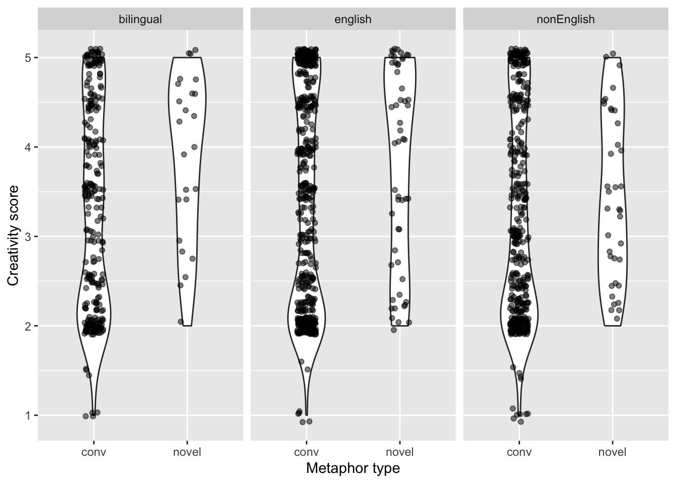
This data is from a metaphor production study. People wrote novel and conventional metaphors, which were then rated for creativity. Speakers were from various language backgrounds.
dat <-read_csv('https://raw.githubusercontent.com/scskalicky/scskalicky.github.io/refs/heads/main/sample_dat/metaphor-data.csv')
Rows: 1304 Columns: 11
── Column specification ────────────────────────────────────────────────────────
Delimiter: ","
chr (5): id, type, sex, hand, language
dbl (6): subject, conceptual, nm, trial, rt, ses

ℹ Use `spec()` to retrieve the full column specification for this data.
ℹ Specify the column types or set `show_col_types = FALSE` to quiet this message.
The first use of the word anova is the ALL CAPS VERSION - ANalysis Of VAriance - (ANOVA), is itself a statistical model. ANOVAs are models which compare means among 3 or more groups or 3 or more levels of a categorical variable in order to test for significant differences among/between groups. They are what you do instead of a t-test when you have more than 2 groups, or when you need to do a “factorial” design (where you have two categorical variables with at least two levels each).
To do an ANOVA, we can use the aov function from the stats library in R:
help(aov)
We fit the model with similar syntax as regressions, putting the y variable (our dependent variable) on the left side of the formula, followed by our fixed effects terms, and then the data that we are using.
# fit the modelm1 <-aov(nm ~ language*type, dat)
Obtain summary of the model:
summary(m1)
                Df Sum Sq Mean Sq F value   Pr(>F)
language         2    8.4   4.216   3.087 0.045992 *
type             1   17.5  17.503  12.815 0.000357 ***
language:type    2    1.6   0.794   0.581 0.559504
Residuals     1298 1772.9   1.366
---
Signif. codes:  0 '***' 0.001 '**' 0.01 '*' 0.05 '.' 0.1 ' ' 1
We see that we have a significant effect of language and type, but that the interaction is not significant.
Let’s conduct pairwise tests on a model without the interaction:
# Tukey Honest Significant DifferencesTukeyHSD(aov(nm ~ language + type, dat))
  Tukey multiple comparisons of means
    95% family-wise confidence level

Fit: aov(formula = nm ~ language + type, data = dat)

$language
                            diff        lwr          upr     p adj
english-bilingual     0.06196624 -0.1363463  0.260278825 0.7438175
nonEnglish-bilingual -0.12056253 -0.3271209  0.085995881 0.3572727
nonEnglish-english   -0.18252878 -0.3556975 -0.009360068 0.0360146

$type
                diff       lwr       upr    p adj
novel-conv 0.4100941 0.1853807 0.6348075 0.000356
That’s nice and all, but in our research we will most likely not use aov to perform statistical tests (although it’s doing the same thing as a regression model, basically). But now you at least know this is one possible meaning of “doing an ANOVA” in R. Let’s explore the other uses.
ANOVA - checking significance of terms
Another type of “anova” in R is to perform an analysis of the significance of terms in a fit regression model. This is done to assess whether the fixed effects of a regression model are “significant” - whether they explain enough additional variance in the outcome variable when considered in light of all the other predictor variables.
To be clear, this is a very different use of “anova” than fitting an ANOVA model! However the overall logic is somewhat similar - these tests provide an omnibus test of significance for a term, telling you whether your five-level categorical variable of language background interacted with your three-level categorical variable of pedagogical intervention is actually making for a better model. Basically, you want to know if the totality of a predictor (rather than any pairwise comparisons within a predictor) make for a significantly better model fit.
So the first thing we will need is to create a regression model. Let’s approximate the above aov analysis, but instead using a linear model:
m2 <-lm(nm ~ language*type, data = dat)
We can obtain a summary of the model. This shows the effects of each variable at its different levels, with significance being determined by whether any particular level / effect meaningfully increases the intercept term.
What we do not see in this output is whether the interaction term or any single main effect term (language or type separately) is or is not “significant”. Moreover, because our language and type terms are interacted, we cannot assess whether their independent effects are significant. This is a common challenge when interpreting dummy-coded variables in a regression output in R (and why we might want to immediately proceed to a post-hoc modelling library such as emmeans()).
summary(m2)
Call:
lm(formula = nm ~ language * type, data = dat)

Residuals:
    Min      1Q  Median      3Q     Max
-2.3571 -1.1938 -0.1071  1.1429  1.8062

Coefficients:
                             Estimate Std. Error t value Pr(>|t|)
(Intercept)                   3.28585    0.07179  45.769   <2e-16 ***
languageenglish               0.07129    0.08847   0.806   0.4205
languagenonEnglish           -0.09201    0.09194  -1.001   0.3171
typenovel                     0.59957    0.24913   2.407   0.0162 *
languageenglish:typenovel    -0.16897    0.30085  -0.562   0.5744
languagenonEnglish:typenovel -0.34071    0.31981  -1.065   0.2869
---
Signif. codes:  0 '***' 0.001 '**' 0.01 '*' 0.05 '.' 0.1 ' ' 1

Residual standard error: 1.169 on 1298 degrees of freedom
Multiple R-squared:  0.01529,   Adjusted R-squared:  0.01149
F-statistic:  4.03 on 5 and 1298 DF,  p-value: 0.00124
We can use an “anova” test to tell us whether each term is significant in the context of the model. There are at least two different flavours of this kind of anova. The first is the anova() function in the stats library. Look at the output - it provides one row per term in the model. One for language, one for type, and one for the interaction term. This is telling us that the main effect of language is just below the threshold for statistical significance, and that the main effect of type is far below the threshold. These do not tell us anything about the within-term contrasts, only that including the overall effect of the term in the model creates a significantly better model.
stats::anova(m2)
Analysis of Variance Table

Response: nm
                Df  Sum Sq Mean Sq F value    Pr(>F)
language         2    8.43  4.2159  3.0866 0.0459924 *
type             1   17.50 17.5033 12.8148 0.0003566 ***
language:type    2    1.59  0.7935  0.5810 0.5595041
Residuals     1298 1772.89  1.3659
---
Signif. codes:  0 '***' 0.001 '**' 0.01 '*' 0.05 '.' 0.1 ' ' 1
P.s., compare this output with the test of the aov model. What do you see?
anova(m1)
Analysis of Variance Table

Response: nm
                Df  Sum Sq Mean Sq F value    Pr(>F)
language         2    8.43  4.2159  3.0866 0.0459924 *
type             1   17.50 17.5033 12.8148 0.0003566 ***
language:type    2    1.59  0.7935  0.5810 0.5595041
Residuals     1298 1772.89  1.3659
---
Signif. codes:  0 '***' 0.001 '**' 0.01 '*' 0.05 '.' 0.1 ' ' 1
However, there are other libraries which let you obtain anova() contrasts. Another is from the car package, and this one spells anova with a capital “A” (Anova()).
With this version of Anova, you can obtain two different types of contrasts.
Type II contrasts are used to identify the significance of terms at a particular level. This means basically testing whether main effects are significant and without considering their presence in an interaction.
The test asks - when controlling for the other variables at the same level, does adding this variable have a significant effect on explaining the outcome?
car::Anova(m2, type ='II')
Anova Table (Type II tests)

Response: nm
               Sum Sq   Df F value    Pr(>F)
language         8.01    2  2.9317 0.0536608 .
type            17.50    1 12.8148 0.0003566 ***
language:type    1.59    2  0.5810 0.5595041
Residuals     1772.89 1298
---
Signif. codes:  0 '***' 0.001 '**' 0.01 '*' 0.05 '.' 0.1 ' ' 1
Type III contrasts are used to test whether all terms are significant in a model while taking into account their presence in an interaction. Notice that we obtain very different results in terms of the significance of type between Type II and Type III tests. This is because the intercept term is now there, which takes on the default values of all terms. In this case, the intercept term represents the bilingual level of language and the conv level of type. We can’t actually make any inferences about the “significance” of these effects based on this output, because we are using dummy-coded variables.
car::Anova(m2, type ='III')
Anova Table (Type III tests)

Response: nm
               Sum Sq   Df   F value  Pr(>F)
(Intercept)   2861.15    1 2094.7595 < 2e-16 ***
language         6.10    2    2.2329 0.10763
type             7.91    1    5.7920 0.01624 *
language:type    1.59    2    0.5810 0.55950
Residuals     1772.89 1298
---
Signif. codes:  0 '***' 0.001 '**' 0.01 '*' 0.05 '.' 0.1 ' ' 1
Note that the anova() function from the stats library does Type I contrasts - which test the iterative inclusion of terms while controlling for other terms.
So basically, if we have an interaction, we want to use Type III, but need to do something extra with out categorical variables (see below). We want to save Type I for comparing iterative terms between two models, and Type II should only be used when we don’t have interactions. (Hrmm…this raises several questions about what we are doing!)
Anoyhow, this brings us to our third use of anova - model comparisons!
anova() comparing nested models
The final use of anova() is to compare two or more models that are nested - what does that mean? Basically, nested models are models that differ by only one term. Using our data, an example of a nested model would be comparing a model with type as a fixed effect against a model with both type and language as fixed effects. The models would differ by only one term: language. We use anova() to test whether the model with the additional predictor is “better”, which in turn means whether the addition of a single predictor makes for a significantly better model fit.
Let’s see how it works:
# fit a regression model with just "language" as the predictormod1 <-lm(nm ~ language, data = dat)
# fit a regression model with language and type as fixed effectsmod2 <-lm(nm ~ language + type, data = dat)
Having fit two models, we can now do a model comparison.
What do you see? Both the models are listed, and the model that “wins” is the model with the lowest RSS (which would be the lowest residual sums of squares) - meaning the model that best predicts the original data.
The inclusion of type makes for a significantly better model fit when compared to a model with just language
anova(mod1, mod2)
Analysis of Variance Table

Model 1: nm ~ language
Model 2: nm ~ language + type
  Res.Df    RSS Df Sum of Sq      F   Pr(>F)
1   1301 1792.0
2   1300 1774.5  1    17.503 12.823 0.000355 ***
---
Signif. codes:  0 '***' 0.001 '**' 0.01 '*' 0.05 '.' 0.1 ' ' 1
Do you notice anything similar in this output? What is going on? Essentially this manual model comparison using a nested model is doing a similar thing as the Anova test on a single model.
car::Anova(lm(nm ~ language + type + language, data = dat))
Anova Table (Type II tests)

Response: nm
           Sum Sq   Df F value   Pr(>F)
language     8.01    2  2.9336 0.053559 .
type        17.50    1 12.8231 0.000355 ***
Residuals 1774.48 1300
---
Signif. codes:  0 '***' 0.001 '**' 0.01 '*' 0.05 '.' 0.1 ' ' 1
We can extend this to test the presence of an interaction
mod3 <-lm(nm ~ language * type, data = dat)
Here we can chain our model comparisons to see effectively the same anova table as running Anova() on a single fully defined model:
anova(mod1, mod2, mod3)
Analysis of Variance Table

Model 1: nm ~ language
Model 2: nm ~ language + type
Model 3: nm ~ language * type
  Res.Df    RSS Df Sum of Sq      F    Pr(>F)
1   1301 1792.0
2   1300 1774.5  1    17.503 12.815 0.0003566 ***
3   1298 1772.9  2     1.587  0.581 0.5595041
---
Signif. codes:  0 '***' 0.001 '**' 0.01 '*' 0.05 '.' 0.1 ' ' 1
This can help us understand the difference between Type II and Type III Anova.
The Type II tests the presence of the iterative addition of each term and gives us the exact same output as model comparisons.
car::Anova(mod3, type ='II')
Anova Table (Type II tests)

Response: nm
               Sum Sq   Df F value    Pr(>F)
language         8.01    2  2.9317 0.0536608 .
type            17.50    1 12.8148 0.0003566 ***
language:type    1.59    2  0.5810 0.5595041
Residuals     1772.89 1298
---
Signif. codes:  0 '***' 0.001 '**' 0.01 '*' 0.05 '.' 0.1 ' ' 1
The Type III contrasts give us the significant of each term when controlling for all the other terms. This means that for categorical variables, the significance of the term is based on controlling for the baseline of other categorical terms (notice that we get an intercept value when using Type III but not Type II)
car::Anova(mod3, type ='III')
Anova Table (Type III tests)

Response: nm
               Sum Sq   Df   F value  Pr(>F)
(Intercept)   2861.15    1 2094.7595 < 2e-16 ***
language         6.10    2    2.2329 0.10763
type             7.91    1    5.7920 0.01624 *
language:type    1.59    2    0.5810 0.55950
Residuals     1772.89 1298
---
Signif. codes:  0 '***' 0.001 '**' 0.01 '*' 0.05 '.' 0.1 ' ' 1
Type II vs. Type III and contrast coding
Exploring the somewhat cryptic warning that car gives in their help about Type II and Type III…
It seems the “correct” way to use a Type III test is when you have some sort of contrast coding that is not dummy coding, such as sum contrast coding. Let’s compare the results of a model with and without such coding applied.
# create a new version of the data, and make dat2 <- dat %>%mutate(type =factor(type), language =factor(language))contrasts(dat2$type) <- contr.sumcontrasts(dat2$language) <- contr.sum
# fit the contrast coded model:m0 <-lm(nm ~ language*type, data = dat2)
Type III Anova for a contrast-coded regression:
car::Anova(m0, type ='III')
Anova Table (Type III tests)

Response: nm
              Sum Sq   Df   F value    Pr(>F)
(Intercept)   4591.4    1 3361.5574 < 2.2e-16 ***
language         5.9    2    2.1528 0.1165694
type            17.4    1   12.7106 0.0003768 ***
language:type    1.6    2    0.5810 0.5595041
Residuals     1772.9 1298
---
Signif. codes:  0 '***' 0.001 '**' 0.01 '*' 0.05 '.' 0.1 ' ' 1
Type III Anova for a dummy-coded version of the same regression - egads.
car::Anova(mod3, type ='III')
Anova Table (Type III tests)

Response: nm
               Sum Sq   Df   F value  Pr(>F)
(Intercept)   2861.15    1 2094.7595 < 2e-16 ***
language         6.10    2    2.2329 0.10763
type             7.91    1    5.7920 0.01624 *
language:type    1.59    2    0.5810 0.55950
Residuals     1772.89 1298
---
Signif. codes:  0 '***' 0.001 '**' 0.01 '*' 0.05 '.' 0.1 ' ' 1
We can see the significance of type in a Type III dummy coded regression is the comparison between type at the default level of language.
emmeans::emmeans(mod3,pairwise ~ type | language)$contrasts
language = bilingual:
 contrast     estimate    SE   df t.ratio p.value
 conv - novel   -0.600 0.249 1298  -2.407  0.0162

language = english:
 contrast     estimate    SE   df t.ratio p.value
 conv - novel   -0.431 0.169 1298  -2.553  0.0108

language = nonEnglish:
 contrast     estimate    SE   df t.ratio p.value
 conv - novel   -0.259 0.201 1298  -1.291  0.1970
Conclusion
The moral of the story is that you probably won’t be using aov, and that using anova() or Anova() to check the significance of your terms is a delicate process. Be really careful when you assume the output of Anova tables is showing you what you think it is showing you. This is another reason I tend to prefer going straight to hypothesis testing with emmeans(), which actually answers research questions. However, there can also be much use in building a good model - one which packs the most punch with the least number of predictors. A model comparison approach works well for such an approach.